The performance of any system can be only as high as the oscillator that defines and maintains its stability. While timing performance, such as stability, drift, aging and Allan deviation, is well-understood, the performance is rarely employed to demonstrate the cost savings that can be achieved.
For example, data centers have thousands of servers and oscillators that can maintain high precision in the presence of shock, vibration, electrical noise, thermal gradients, acceleration and pressure, which can significantly reduce the total cost of ownership. To understand how such tiny devices deliver such impressive results, let’s delve into their characteristics and focus on the characteristics of the data centers themselves.
The distributed database is arguably the most common function within most data centers. As an example, we can use the ubiquitous Excel spreadsheet, which in the case of a data center would be a truly massive document. For the purposes of our illustration, let’s assume we are both bidding on an item on eBay, and it turns out that our bids are equal and appear on the eBay server at about the same time. Who gets the product: you or me?
Keep in mind that in a data center, the spreadsheet can be stored on different servers or even different regions of the data center, which itself can be distributed geographically worldwide. In Figure 1, the red columns (including my bid) are stored on Server A, those in blue (including your bid) are stored in Server B and another section for reference resides on Server C. To access them, the data center generates east-west traffic, which is the transfer of data packets between servers within a data center. East-west traffic represents at least 70% of data center traffic, so reducing its amount is very important.

Figure 1: A distributed database divides its content into multiple regions in a data center. (Source: SiTime Corp.)
In our case, the bids appear so near in time that small fractions of time make the difference between who wins. In Figure 2, we show two scenarios: Packet A that represents my bid and Packet B that represents yours. In both cases, the timestamp when the bid arrives is surrounded by a “window of uncertainty” (WOU), which is essentially the error bars of the timestamp. In Scenario 1, the WOU overlaps, requiring the servers to generate more east-west traffic to break the tie, while in Scenario 2, the WOU is narrower, so no overlap occurs and therefore no east-west traffic needs to be generated to break the tie. Scenario 2 creates a more efficient data center.
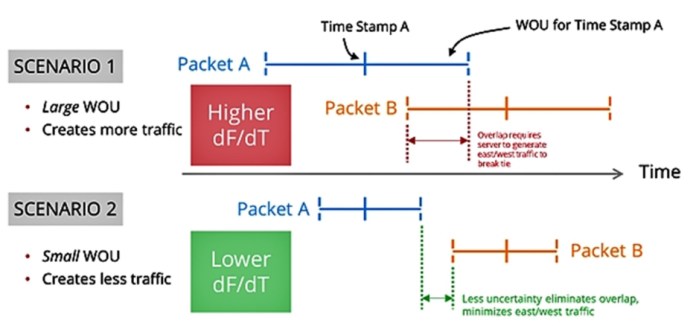
Figure 2: Minimizing uncertainty eliminates overlap and contributes to increased server utilization. (Source: SiTime Corp.)
So how is WOU related to oscillator performance? To understand this, we need to understand the source of WOU. Figure 3 shows a typical IEEE 1588 precision time protocol (PTP) servo loop. At left, the network traffic timestamps are extracted from the packet to steer a servo loop whose goal is to filter the timestamp and extract the “lucky” packet. This low-pass filtering reduces the packet delay variation (PDV) entering the network to extract the packet. During this filtering process, the job of the local oscillator (LO) is to maintain stability between servo updates. Every time a new timestamp appears the LO will update the loop. However, between the updates, the job of the LO is to maintain short-term stability for the client.

Figure 3: A typical IEEE 1588 PTP servo loop (Source: SiTime Corp.)
The goal is to reduce the bandwidth of the loop filter to reduce the PDV from the network. The narrower the servo bandwidth, the more PDV that can be eliminated and the more accurate the timestamps will be. But reducing the bandwidth simultaneously increases the amount of undesirable LO noise appearing at the client. So the goal is to reduce the loop filter bandwidth only to the specific point where the noise at the client is at a minimum. So where does precision timing play a role? We’ll discuss that next.
The banner spec conundrum
It’s interesting to note that when evaluating precision timing, the banner datasheet specification is “frequency-over-temperature stability” in units of parts per million or parts per billion (for example, 1 ppm or 0.5 ppm or 100 ppb). This is the first thing people think of when selecting a precision time device. However, in PTP applications, the LO is disciplined to network timing and frequency changes (in the oscillator) that are slower than the servo’s update rate and are filtered by the servo loop (because the oscillator’s noise is high-pass–filtered by the servo loop).
Thus, an oscillator’s frequency-over-temperature specification, which is guaranteed over the lifetime of the oscillator, isn’t a critical parameter here. What is critical is the short-term stability resulting from changes in temperature—and by short term, we mean the time between servo loop updates (or 1 over the servo-loop’s bandwidth, which is the loop’s time constant).
The way we quantify an oscillator’s temperature sensitivity is using a “frequency-over-temperature slope” specification, which we’ll refer to more simply as ΔF/ΔT (that is, the derivative of frequency with respect to temperature). This ΔF/ΔT datasheet specification quantifies the oscillator’s change in frequency with changes in temperature and has units of parts per billion per degrees Celcius. An ideal curve is a horizontal line centered at 0 on the y-axis, meaning the output frequency doesn’t change with temperature. However, in practice, ΔF/ΔT is non-zero.
Evaluating Figure 4, the better “datasheet” stability specification is Device 2, as it exhibits ±50-ppb frequency-over-temperature stability compared with ±100 ppb for Device 1. However, in PTP applications, the better oscillator is actually the one that has a more gradual frequency-over-temperature slope. So here, the ±100-ppb device provides better PTP performance, which can be counterintuitive.
To summarize, while the banner datasheet specification for precision timing is frequency-over-temperature stability, the actual determinant of performance in a data center (and other synchronization applications) is short-term stability that is dominated by thermal drift and reported in datasheets as ΔF/ΔT.
The banner datasheet specification does not apply to network synchronization because it is a lifetime specification over 10 years. But 10 years doesn’t matter for a servo loop that is disciplined to the network multiple times per second.
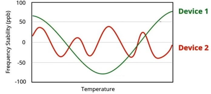
Figure 4: Performance over a device’s lifetime has little meaning in short periods of time. (Source: SiTime Corp.)
In short, an oscillator with lower ΔF/ΔT delivers more accurate timestamps, and more accurate timestamps create less east-west traffic. And as less traffic translates into higher server utilization, it is possible to reduce the number of servers in the data center. And fewer servers mean lower capital expenses and operating costs, which increases operator profits. The more impressive oscillator would be one that has a more gradual frequency slope over temperature (Device 1), even though it may not have less peak-to-peak variation over its lifetime. In short, low sensitivity to temperature changes rather than lifetime peak-to-peak stability is the critical oscillator parameter for synchronizing networks.
Comparing quartz and MEMS oscillators
Crystal oscillators have been used as a timing reference for many decades, and while they have been improved over time, the inherent limitations of quartz-based timing technology can never be fully mitigated. MEMS-based oscillators have none of these stability problems and were created to overcome the limitations of quartz. They are inherently rugged, making them uniquely suited for extremely harsh operating environments, as their structure is fabricated from a single mechanical structure of single-crystal silicon.
SiTime uses a process called EpiSeal to clean the resonator and hermetically seal it in a vacuum, which effectively eliminates aging. Their mean-time-before-failure rate is 1.14 billion hours, which is about 30× greater than crystal oscillators.
From the perspective of stability, the two architectures are very different. For the quartz TCXO (Figure 5), temperature sensing is performed on the quartz itself, with the sensor physically separate and located below the quartz, which creates a thermal lag during thermal gradients. Therefore, the device can track only very slow temperature changes.
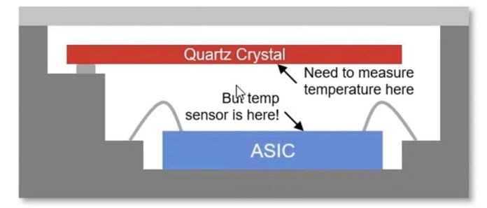
Figure 5: Quartz oscillators suffer thermal lag due to the temperature sensor located far away from the quartz membrane. (Source: SiTime Corp.)
In contrast, the SiTime MEMS TCXO (Figure 6) uses two MEMS resonators fabricated next to each other on the same silicon die. The top resonator provides a very stable timing reference with temperature changes, while the bottom resonator acts as a temperature sensor. As both MEMS resonators sit next to each other, any change in temperature across the top MEMS resonator is observed by both resonators at the same time, and across the bottom MEMS resonator, and the ratio of the two output frequencies (one derived from each resonator) provides a measure of temperature change that is used to correct the output frequency with very high update rates. Therefore, the device can easily track rapid temperature changes.
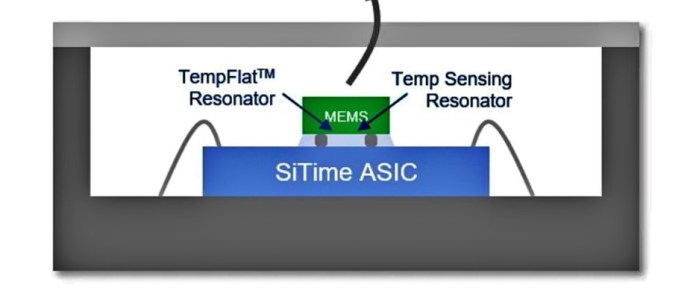
Figure 6: The tighter integration inherent to MEMS technology improves thermal measurement and tracking. (Source: SiTime Corp.)
Show me the money
Let’s consider a scenario to represent the benefits that MEMS-based precision timing can produce in a data center (Table 1). In this case, the facility has 300,000 servers per building and three buildings per campus. Every four years, the servers are refreshed, and the total cost of ownership for each server is about $200/month. If we can achieve just a 1% increase in server utilization, the annual savings would be $1.8 million for each building and $5.4 million for the entire campus.
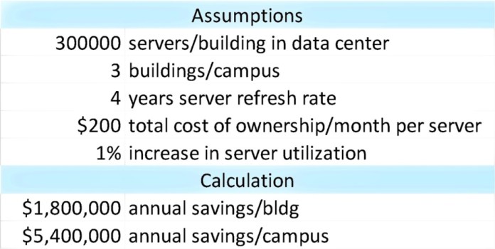
Table 1: MEMS-based precision timing can save an average data center $5 million annually. (Source: SiTime Corp.)
The above scenario may be conservative and even greater increases in server utilization can be achieved. Because designers often use traditional datasheet specifications when selecting oscillators, the potential for upside is significant. That said, it’s important to consider the intended application when selecting an oscillator because, as we demonstrated in the data center scenario, a single “banner spec” alone can be irrelevant and even degrade system performance.
About the author
 Gary Giust heads technical marketing at SiTime, where he enjoys participating in industry standards, architecting timing solutions and educating customers. Prior to SiTime, Giust founded JitterLabs and previously worked at Applied Micro, PhaseLink, Supertex, Cypress Semiconductor and LSI Logic. Giust is an industry expert on timing, has co-authored a book and is an invited speaker, an internationally published author in trade and refereed journals and a past technical chair for the Ethernet Alliance’s backplane subcommittee. He holds 20 patents. Giust obtained a doctorate from the Ira A. Fulton Schools of Engineering at Arizona State University, Tempe; a master of science from the College of Engineering & Applied Science at the University of Colorado Boulder; and a bachelor of science from the College of Engineering and Physical Sciences at the University of New Hampshire, Durham, all in electrical engineering.
Advertisement
Learn more about SiTime