Improving DDS signal generation using interpolation

BY DEREK SONG,
Siglent Technologies America
www.siglent.com

The term “Interpolated DDS Technique,” used to describe the operating principle behind some of today’s arbitrary waveform generators, may be unfamiliar or confusing to some engineers, even experienced users of function generators. To explain the meaning of this term and to discuss its advantages, let’s compare traditional direct digital synthesis (DDS) with Interpolated DDS.

Traditional vs. Interpolated

In the basic design of the traditional DDS technique (Fig. 1 ), digital waveform data is output at intervals determined by the frequency of the DDS circuitry’s reference clock. Each of these discrete data samples is then converted consecutively by a D/A converter using the same clock. That is, in a traditional DDS structure, the clocks for the DDS and for the D/A converter run at the same frequency. 

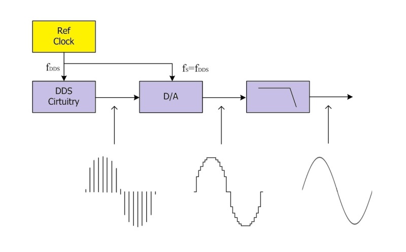
Fig. 1: In a traditional DDS structure, the output of a DDS circuit controlled by a reference clock is fed to a D/A converter controlled by the same clock. The D/A’s output is smoothed by a reconstruction filter.

The output of the D/A converter is then fed to a reconstruction filter, which smooths the discrete step values of the D/A’s output to produce a more continuous “analog” signal.

In an Interpolated DDS system (Fig. 2 ), the major difference is that an interpolator is inserted between the DDS circuitry and D/A converter. In this structure, digital waveform data is output in response to reference clock of the DDS circuitry, interpolated by some numerical factor, I, which thus increases the number of discrete digital waveform data samples by a factor of I.

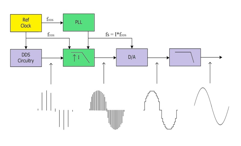
Fig. 2: The structure of an Interpolated DDS system includes two extra elements: a phase-locked loop (PLL) and an interpolator, shown here in green. 

The resultant digital data is then converted by the D/A, which is now clocked by a sampling clock whose frequency is “I” times the frequency of the DDS reference clock. As with the traditional DDS, a reconstruction filter is applied to the D/A converter output.

As a real-world example of how this works, consider the Interpolated DDS technique as it is applied in the Siglent SDG2000X. The SDG2000X uses an interpolation factor (I) of 4, and because the reference clock of the SDG2000X’s DDS circuitry is 300 MHz, the frequency of the sampling clock of the D/A is increased to 1.2 GHz. Thus the D/A outputs at a sample rate of 1.2 Gsamples/s.

Breaking the bandwidth limit

While the preceding paragraphs explain the mechanics behind the interpolated sampling technique, the question remains: “Why use this unique sampling technique?” To answer, let’s first make a time-domain comparison of the output of the D/A using two sample rates. 

Looking at the output waveform of the D/A, the interpolated, 1.2-Gsamples/s sample rate results in smaller steps (higher resolution) than with the 300-Msamples/s sampling clock (Fig. 3 ).

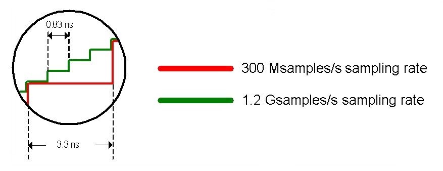
Fig. 3: The interpolator increases the number of samples sent to the D/A by of factor of I, working at a sampling clock frequency created by a PPL that is I times the basic DDS reference clock frequency; for the case shown above, I = 4.

You may think, “If both waveforms are to be passed through a reconstruction filter to smooth the steps, then the sample rate shouldn’t matter.” But the step size does affect the final smoothed waveform.

To get a clearer understanding of why, let’s look at the two waveforms in the frequency domain. Consider an example in which a sine wave with a frequency of 80 MHz (f_out ) is produced by a traditional DDS using a D/A clocked at a sampling frequency (f_s ) of 300 MHz. The spectrum of the D/A’s output (Fig. 4 ) includes the fundamental frequency (f_out ), and its image frequencies, (N x f_s ) ± f_out , where N = 1, 2, … . Amplitudes of all the spectrum components comply with the sin(x)/x envelope.

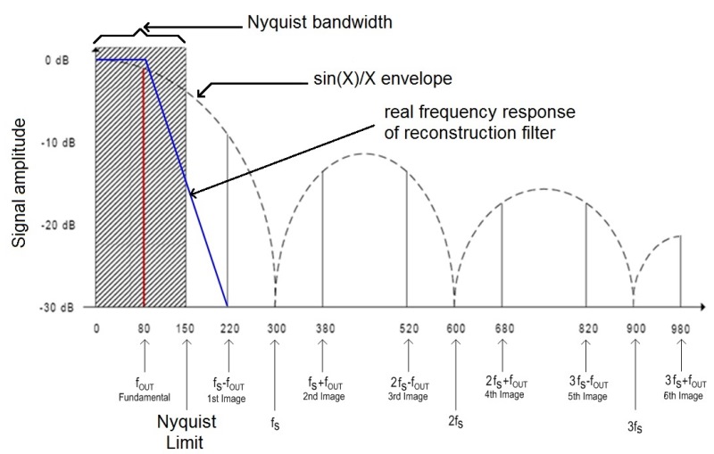
Fig. 4: The diagram above shows the spectrum of an 80-MHz waveform created by a traditional DDS with a 300-Msamples/s A/D converter.

To smooth the waveform, the reconstruction filter must ideally filter out all the image frequencies located outside the band from 0 Hz to half the sampling frequency — that is, outside the Nyquist bandwidth — and retain all the signals whose frequencies are located within the Nyquist bandwidth. In other words, the filter’s frequency response should coincide with the Nyquist bandwidth (the shaded area in Fig. 4 ). In this case, the maximum frequency of the signals retained can reach the Nyquist Limit (that is, half the sampling-clock frequency).

Of course, in engineering, an ideal filter with a “brick wall” response (complete signal attenuation above a specific frequency with no attenuation before that frequency) doesn’t exist. In the real world, filters actually have some degree of roll-off. (Note that in Fig. 4 , the nearest image occurs at 220 MHz so, for the roll-off slope shown in blue, roll-off should begin at 140 MHz to ensure maximum attenuation.)

But if the output waveform had a frequency of 149.5 MHz rather than 80 MHz, the nearest image would be at 150.5 MHz (1f_s  − f_out ) and the space remaining for roll-off would be 1 MHz, impractically almost a brick-wall filter and not realizable. Generally, the bandwidth limit of a reconstruction filter is 40% of the sampling clock. So for a 300-Msamples/s D/A, the maximum available output frequency would be 120 MHz.

In Fig. 5 , two roll-offs calculated for a ninth-order elliptic reconstruction filter are plotted. The difference is that the calculation for the plot on the left uses ideal components, and the one on the right uses real-world components, with parasitic parameters. As shown, a real filter has an extra ~3 dB attenuation on the corner frequency (120 MHz), and its attenuation performance on the stop-band cutoff frequency (~180 MHz) degrades (~18 dB).

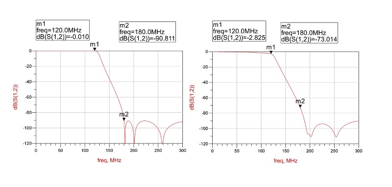
Fig. 5: The plot of the calculated performance of a ninth-order elliptic reconstruction filter with ideal components (left) is significantly different than one using real components with parasitic parameters.

In addition, the sin(x)/x envelope of the D/A’s response itself will add attenuation to the signal. At 40% of the sampling clock, the attenuation caused by the D/A is about 2.4 dB. An inverse sin(x)/x filter is generally necessary to compensate for this attenuation.

Now consider the case for an Interpolated DDS that uses a sampling rate for the D/A of 1.2 GHz (1.2 Gsamples/s) to produce an 80-MHz signal. The nearest image is 1.12 GHz (1.2 GHz − 180 MHz), so the maximum roll-off of reconstruction filter could be 1.04 GHz (Fig. 6 ), and the design of the reconstruction filter is greatly simplified (Fig. 7 ).

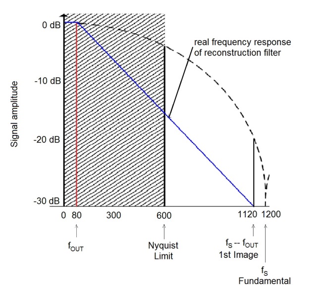
Fig. 6: For the above spectrum of an 80-MHz output, the waveform was generated using Interpolated DDS generator with a 1.2-Gsamples/s D/A converter; note how the reconstruction filter’s roll-off can be relaxed.

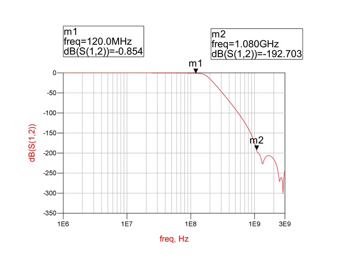
Fig. 7: A real reconstruction filter design with roll-off from 120 MHz to 1.08 GHz is much easier to achieve than one with roll-off from 120 to 180 MHz.

On the other hand, as the main lobe width of the sin(x)/x envelope increases, the attenuation contributed by the D/A decreases. At 120 MHz, the attenuation caused by the 1.2-Gsamples/s D/A is about 0.14 dB, which can be ignored in most cases. Hence, no inverse sin(x)/x filtering is needed.

Based on the above, because of the limits of the reconstruction filter, a 300-Msamples/s D/A can output only a 120-MHz maximum frequency. But a 1.2-Gsamples/s D/A can achieve a higher upper frequency limit. Of course, in the interpolated DDS structure, the digital filter in the interpolator will restrict the frequency to the Nyquist limit of the DDS clock (say 150 MHz), but a digital filter is much easier to design than an analog reconstruction filter. Using the interpolated DDS, it is easy to raise the upper limit of output frequency from 120 MHz to 130 MHz or more.

Avoiding spurs

Spurious signals due to intermodulation distortion are unavoidable in a D/A converter. In a traditional DDS structure, it is difficult to remove some intermodulation distortion components, referred to as spurs, between the clock and the output signal, such as the spurs at f_s  − 2f_out and f_s  − 3f_out . With a 120-MHz output frequency and 300-Msamples/s sampling rate, the f_s  − 2f_out distortion for a traditional DDS thus occurs at 60 MHz (Fig. 8 ), thus falling into the reconstruction filter’s pass band. It cannot be removed.

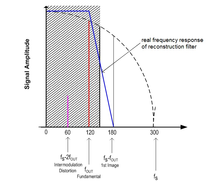
Fig. 8: The intermodulation distortion between the frequency of the generated output signal and the reference-clock frequency cannot be filtered out if it falls within the Nyquist bandwidth.

But with an I = 4 interpolated DDS structure, for a 120-MHz frequency output and 1.2 Gsamples/s, the distortion components f_s  − 2f_out is at 960 MHz and f_s  − 3f_out is at 840 MHz, far outside the reconstruction filter’s pass band. So in the case of the interpolated DDS, spurs don’t affect the final output waveform.

References

• Analog Devices, A Technical Tutorial on Digital Signal Synthesis, http://www.analog.com/media/cn/training-seminars/tutorials/450968421DDS_Tutorial_rev12-2-99.pdf
• A.V. Oppenheim, R.W. Schafer, J.R. Buck, Discrete-time Signal Processing, 2^nd Edition, https://ie.u-ryukyu.ac.jp/~asharif/pukiwiki/index.php?plugin=attach&refer=Frontiers%20of%20Engineering&openfile=Discrete.Time.Signal.Processing.2nd.Ed.Oppenneim.pdf 

Advertisement

Learn more about Siglent Technologies America, Inc