BY PUSHKAR PATWARDHAN
Design Engineering Architect, Cadence Design Systems
www.cadence.com
Automation in automotive electronics has driven the next leap of innovation in transportation, fueled by a fundamental premise: In automotive applications, vehicles must be able to sense their environment accurately.
Indeed, cars must accurately sense not only their own distance, speed, and direction, but also the distance, speed, and direction of any object that could cross their path. Radar is the best way to gather that data, and these automotive systems must successfully interpret the data to make life-and-death decisions.
How radar works
To find out whether there is an object nearby that may affect the car, the automotive system must determine direction or angle of arrival (AoA), speed and distance of the object, and whether the object detected is real or a “false positive” from noise or clutter in the background. Fig. 1 shows how the radar data is gathered.
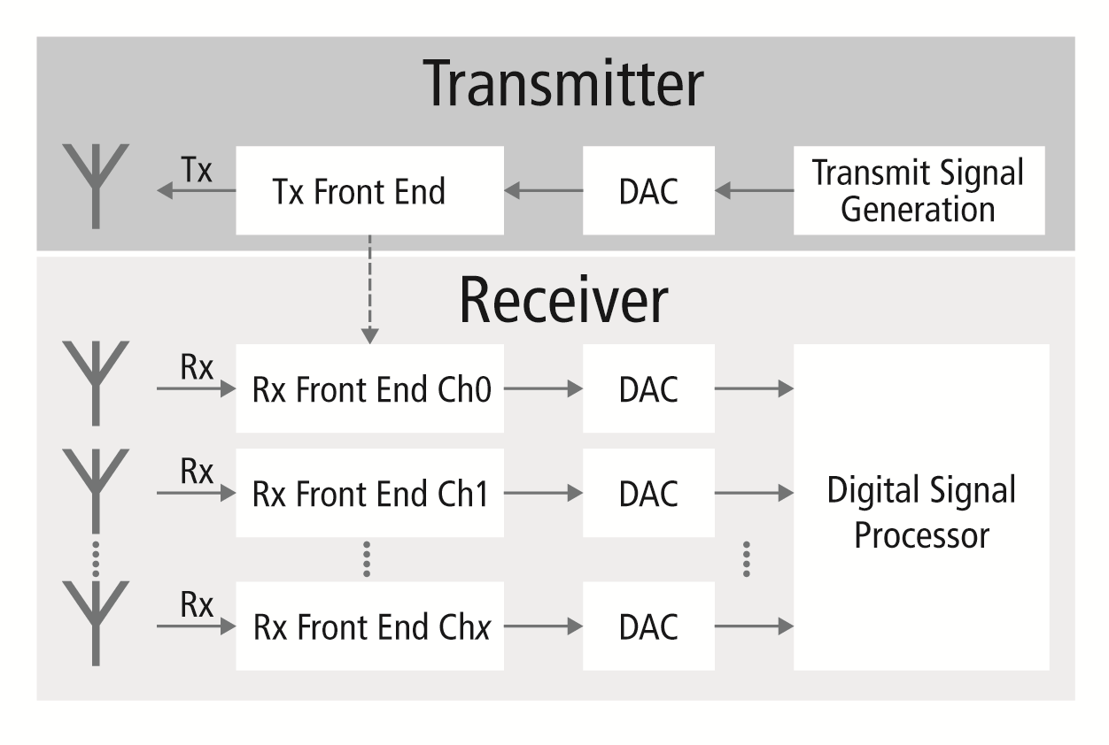
Fig. 1: Block diagram of a radar system.
- A digital transmit signal is generated and converted into analog format and the transmitter signals (TX).
- These signals are released from the transmit antennas and into the environment.
- The signals “bounce” or reflect back to the receiver (RX) and are converted back into digital data by an analog-to-digital converter (ADC).
- The data is then processed by the digital signal processor (DSP) to make decisions based on that data.
DSP: determining whether to stop
The values that influence the decision-making process performed by the DSP include three main factors, as shown in Fig. 2 :
- Direction: In the processing flow, the samples from the input data cube are filtered using a spatial beamforming filter to create digital beams as a part of the digital beamforming (DBF) module.
- Speed and distance: These beams are further processed by a 2D fast Fourier transform (FFT) algorithm along the range and Doppler axis.
- CFAR: Constant false alarm rate, or CFAR, works as a “filter” to determine whether a detected object is likely to be a real object or is part of the background “noise.”
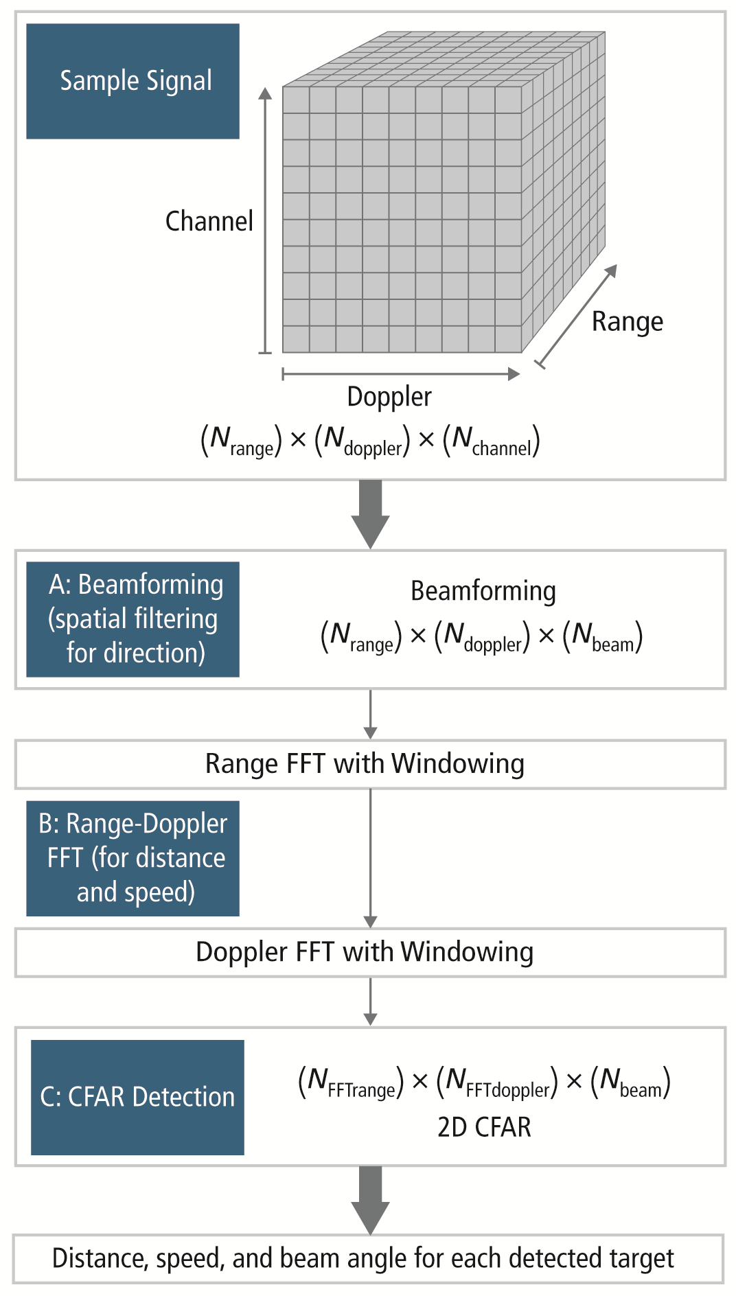
Fig. 2: The DSP block diagram and flow.
For an efficient implementation, the processor must perform data processing and data transfers concurrently. The software should be structured to minimize the data transfers, and the direct memory access (DMA) should be used to perform the data transfers concurrently with module computations.
A. Beamforming for direction
The DBF kernel performs finite impulse response (FIR) filtering along the channel dimension in the data cube. The length of the FIR filter is equal to the number of antenna elements — eight, in this case — and the FIR taps are pre-chosen to pass signals from a beam centered on a particular pre-determined spatial direction and to suppress signals from other directions.
In practice, the DBF processes the data cube as input and produces a range-Doppler 2D signal as an output beam. Different sets of FIR taps can be used to generate multiple beam signals using the same data cube. In this example, five beams are generated along different directions using separate sets of FIR taps.
B. Doppler and range FFT for speed and distance
The radar uses a 2D frequency-domain spectrum in the range-Doppler dimensions for its processing. This spectrum is obtained by performing a 2D FFT — 1D FFT along the range dimension, followed by 1D FFT along the Doppler dimension — and, thus, forming the cube shown in Fig. 2 .
The 2D range-Doppler FFT kernel is used to transform each of the five 2D beam signals produced by the DBF kernel to a 2D frequency-domain spectrum. A windowed 2D FFT is used to separate the signals, with the range FFTs along the range dimension, followed by Doppler FFTs along the Doppler dimension. Each 1D FFT also uses a Hamming window.
The range FFT is computed as a 1D FFT, whereas the Doppler FFT is performed as a block-based FFT to avoid transposing the input and output. The FFT algorithm is based on the Kronecker product-based formalization. In the last stage, the Doppler FFT kernel computes a point-wise energy of each bin.
C. CFAR for target detection
The role of the CFAR is to determine the threshold, above which any return can be considered to probably originate from a target. If this threshold is too low, then more targets are detected at the expense of increased numbers of false alarms.
Conversely, if the threshold is too high, then fewer targets are detected, but the number of false alarms is also low. In most radar detectors, this threshold is determined algorithmically to calculate the probability of a false alarm — or equivalently, false alarm rate or time between false alarms.
The CFAR kernel operates on a 2D energy signal in the frequency domain, classifying each bin or cell under test (CUT) in the 2D FFT energy signal either as a target (positive) or noise/clutter by comparing each CUT with a scaled estimate of noise and clutter. The scale factor and threshold used are determined by the probability of false alarm, or CFAR.
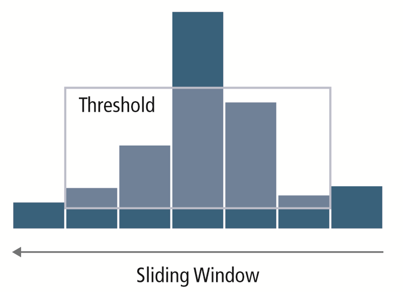
Fig. 3: The CFAR diagram showing positive result and detection exceeding the threshold.
In Fig. 3 , the well-modulated CFAR is the threshold, and the “positive” is where the detection exceeds the threshold. In other words, to determine a target, the value of the CUT is compared with the CFAR — the threshold calculated to determine the levels of the noise floor around the CUT.
CFAR is computed by examining a block of cells around the CUT (Fig. 4 ). To avoid corrupting this estimate with values from the CUT itself, cells adjacent to the CUT, or guard cells, are normally ignored. A target is declared present in the CUT if its value is greater than all of its adjacent cells — CFAR or noise-and-clutter threshold.
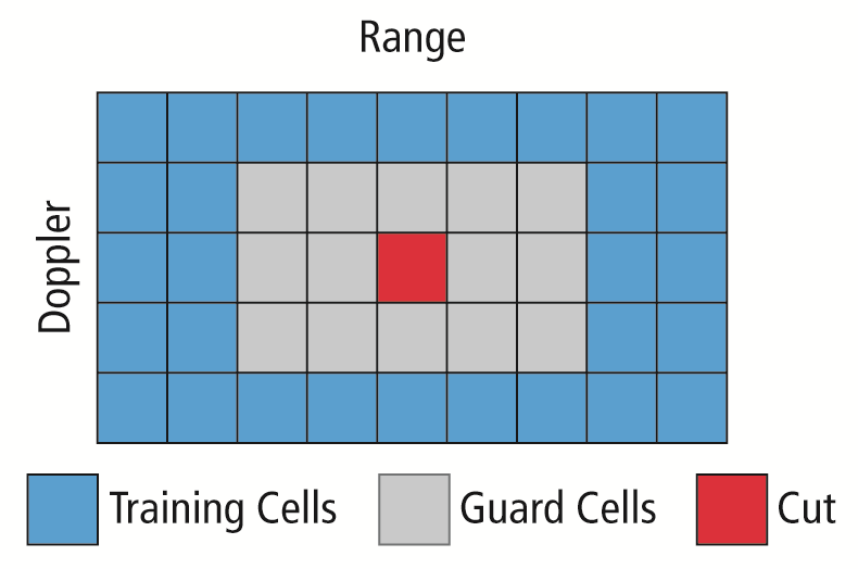
Fig. 4: The CFAR block processing.
CFAR kernels are distinguished by how the noise estimate is formed using the training cells. For example, the cell-averaging constant false alarm rate (CA-CFAR) noise estimate is formed by averaging the values of the cells in the training area, whereas the ordered statistic constant false alarm rate (OS-CFAR) noise estimate is formed by sorting the training area’s cell values in descending order, and using the Nth sorted value.
Combinations of CA-CFAR and OS-CFAR can also be used. The AND CFAR combination performs a logical AND of the classification outcomes of the CA-CFAR and OS-CFAR for each CUT, while the OR CFAR combination does a logical OR.
DSP: the decision maker
When direction, speed, distance, and CFAR have been computed, the DSP will be able to determine whether the ball thrown by a kid from a playground and into the path of an oncoming car is likely to intercept the vehicle in its current trajectory and whether evasive action must be taken. In other words, the embedded system will help make the entire vehicle safer for everyone.
Advertisement
Learn more about Cadence Design Systems