Why care about a scope’s update rate?
While there is no standard definition for oscilloscope update rate, users are at risk if they don’t understand its impact
BY MATT HOLCOMB
System Architect, InfiniiVision oscilloscopes
Agilent Technologies
www.agilent.com
Technology in today’s digital oscilloscopes enables them to process more triggers per second than even the highest-end analog oscilloscopes. The industry buzz phrase for this is “update rate” — but what does that really mean? Since there isn’t an IEEE standard definition of “update rate” for an oscilloscope, this article explains what it is and what the benefit are to the scope user.
Update rate defined
In the infancy of digital sampling oscilloscopes (DSO), update rate was measured in the number of “dots per second” drawn on the display. Each “dot” was one A/D converter sample. The more dots lit up, the more A/D samples getting to the screen.
But that’s only half the story. If a scope collects billions of samples per trigger, and then takes dozens of seconds to get them on the screen, just how many additional triggers are missed? Is your device-under-test politely waiting for your scope to finish before generating the next glitch? Probably not.
So, another metric for update rate could be “how many triggers per second does the oscilloscope draw on the screen?” The goal is to choose just enough samples to plot per trigger, so that by the time you get to the right edge of the display, you’re ready to start the next set. The length of time the acquisition side of the scope needs to wait for the display side is referred to as “blind time.” Not surprisingly, less waiting time is better. But if you’re only getting a few samples per trigger sent to the display, you can be sure that your glitch is hiding between these samples (see Fig. 1 ).
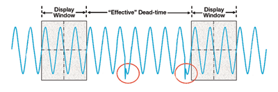
Fig. 1: As a signal moves from probe tip to the oscilloscope display, there are two signal anomalies that are not captured because they happen during the blind, or dead, time. The faster the waveform update rate, the lesser the blind time, giving a higher probability of capturing such events.
All too often, banner specifications on oscilloscope products focus on one of these two aspects of update rate while neglecting the other. The highest fidelity displays, however, are achieved in systems which combine a high number of triggers per second with a high number of points per waveform. In the best of all possible worlds, scopes would provide this performance all the time, in every mode.
There’s more to waveform display than lighting up pixels as fast as the architecture allow. All modern oscilloscopes use a gray-scale canvas to paint their pictures. Areas on the screen that are brighter should represent where the input signal statistically spent more time. This is referred to as “intensity gradation.” The input signal isn’t a collection of discrete samples it’s a continuous waveform.
Dots were viewed as a necessary condescension of yesterday’s digital oscilloscope. But today, the A/D samples on your scope shouldn’t be drawn on the screen as dots: they should be drawn as connected lines, or vectors. Data is processed and rendered as line segments, not as discrete points. And these vectors (which connect equally spaced samples of the input) are of varying lengths. [One example of scopes designed as vector processors is Agilent’s new InfiniiVision X-Series, which plots over a million waveforms/s. See http://tiny.cc/infiniivisionfor a description of these scopes. — ED ]
Statistically speaking, the longer vectors the ones with the higher slew rates indicate where the input signal didn’t spend as much time, and so should be drawn on the display more dimly than the shorter vectors. Consequently, each line segment has a brightness, as well as length and location (see Fig. 2).
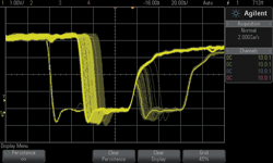
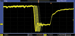
Fig. 2: With intensity gradation, the brighter areas are where points occurs statistically more often than in the dimmer portions. The screen photo at left, taken from an InfiniiVision 3000 X-Series with an update rate > 1,000,000 waveforms/s, intensity gradation shows Infrequent glitches and signal jitter captured after 1 s. Even after 40 s, the screen at from another oscilloscope at right never sees the glitches and shows limited signal jitter due to a much slower update rate.
Update rate’s importance
If you happen to probe a signal, and there was a “glitch” wandering around on that signal, you’d want to see it. But more than likely, you’re looking at, say, a particular trace on your printed-circuit board to make some sort of measurement. Maybe you’re interested in the high and low voltage levels, what the rise time is, or how much timing margin your signal has. Automatic measurements and cursors are great for that.
But the story doesn’t end there. In an unquantifiable way, you take a look at your signal and observe the signal fidelity just how “good” is the signal you’re measuring? Is it noisy? Is it stable? Is it a high more often than a low? How much more often? Do you recognize the interference pattern in the baseline noise? In an instant, you make the analysis in your mind, then a judgment, and then move on to the next signal.
It’s in this mode the transfer of information from the probe tip to the display to your brain where update rate is critically important. If your scope is rendering this information poorly, due to slow waveform update rate, then it’s blind to you during a long portion of the time you are debugging. In addition to what an oscilloscope with slow update rate will miss due to its blind time, a fast plotter provides a really smooth “feel” to the scope. As traces are moved around on the display and you need to change the time base or make additional changes to the scope, you will not have to wait for the scope to respond. Some oscilloscopes with slow update rate take seconds to respond. In that time, you are not sure if the instrument has locked up or if it is capturing data anymore.
Beware the ‘special’ mode
Maybe you want to filter away, or perhaps emphasize, certain aspects of your input signal. You provide this hint to your scope by the mode you set it in. If you really want the rare events drawn more brightly (and not miss any of them, if the scope needs to decimate away data), you probably want to turn on “peak detect” mode. If you really don’t care about the high-frequency fuzz on the signal, but rather want to see how it’s trending, you probably turn on some sort of averaging mode (sometimes called “high-resolution” mode).
Additionally, you might want to use some of the scopes advanced analysis features (automatic measurements, mask testing, and so on) to help you evaluate your signal’s quality. Perhaps you’ve turned on your mixed-signal oscilloscope’s logic channels, for additional context of what’s going on, or to help you triggering precisely where you want.
Does enabling these “bonus features” reduce the update rate of your oscilloscope? In other words, how much information transfer do you lose when actually try to use your scope versus when it’s set at the specification listed by the asterisk in the datasheet.
The hallmark of a genuinely useful “signal visualization instrument” is that it continues to do the job you bought it for regardless of how you set it up. This can’t be emphasized enough. Any feature is of no use to you if you don’t (or can’t) use it when viewing your input signals. Do you disable your scope’s deep memory because it cripples the plot rate? Does turning on a measurement turn off fast-plotting? Are performance tradeoffs common, evident, and painful?
Once you’re confident that your scope will be there with you during your debugging needs, you’re on a journey of a long and lasting benchtop friendship. It is important to evaluate an oscilloscope before you make a purchase. Choosing one with the highest update rate could save you weeks of debug time because you will see more of your signal more of the time. ■
Advertisement
Learn more about Agilent Technologies